4.1. Magnetics
Magnetics are found in filter subsystems, where they integrate voltage ripple to provide limited current ripple. Depending on the filter, magnetics describe either a single inductor or a set of several identical inductors.
4.1.1. The “Simple L” inductor(s) magnetics model
This magnetics model is the simplest available, describing one or several identical inductors with basic electrical values: inductance and series resistance.
4.1.1.1. Models and assumptions
4.1.1.1.1. Loss
The only loss mechanism is resistive power loss due to series resistance (no attempt is made to model AC winding or core losses).
4.1.1.1.2. Cost
The total cost is computed as \(Cost = n_{par} \left( Cost_{constant} + Mass \times Cost_{material} \right)\)
4.1.1.2. Design algorithm in auto design mode
The auto-design approach for the “simple” magnetic model is as follows:
inductance is chosen as required by the filter design
series resistance is chosen so the resulting resistive power loss will be \(P_{loss} = P_{transfer} \times loss factor\)
volume is then computed as \(Volume = n_{par} \times K_{volume} \times \left(L_{phase} \times I_{max\:rated} \times I_{rms\:rated}\right)^α\)
mass is derived as \(Mass = Volume \times Density\)
For an inductor, \(L \times I_{max} \times I_{rms} \sim A_c \times A_w\) which means that \(Volume \sim \left( A_c \times A_w \right)^α\): dimensional analysis explains the default value of 3/4 for \(α\).
Typical values of \(K_{volume}\) can be derived from off-the-shelf or existing components:
For small off-the-shelf inductors (a few µH to a few 100 µH) with low currents (a few amps to 10 amps), typical value range goes from 4e-4 to 1e-3.
For larger inductors, as it strongly depends on the technology and the manufacturer process, value range is much wider (between 4e-4 and 4e-3) and has to be carefully chosen by the designer.
4.1.2. The “Custom EE inductor(s)” magnetics model
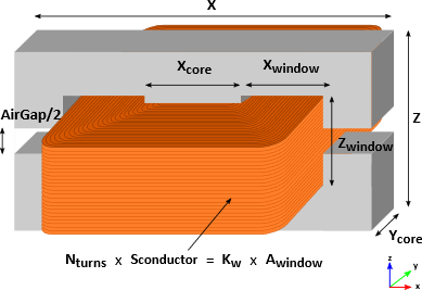
This magnetics model describes one or several identical ‘custom-built’ inductors, each composed by:
an EE magnetic core,
a foil winding.

4.1.2.1. Model and assumptions
4.1.2.1.1. Magnetic circuit
Induction is assumed homogeneous across the cross-section of each leg of the core. The air gap is modeled with cross-section equal to core leg’s (i.e. no fringing). This gets less and less valid when the air gap increases.
4.1.2.1.2. Window fill factor
The window fill factor \(\frac{A_{conductor}}{A_{window}}\) defines indirectly the total conductor cross-section. Typical values for this are:
Full winding: between 30% and 45% for round winding or between 45% and 60% for foil winding. These values are normally a reasonable trade off between fully utilizing the space available for a given core size, while avoiding excessive manufacturing cost.
High fill: up to about 65% for round winding and 80% for foil winding. These values are achievable, but generally only with special expensive measures, such as completing each coil by hand after the residual hole becomes too small to fit the winding shuttle.
4.1.2.1.3. Thermal
No electrothermal coupling is taken into account. Because all loss mechanisms normally increase with temperature (over the temperature range of interest) actual losses should be lower than estimated and actual temperatures somewhere between calculated and maximum permissible temperatures.
4.1.2.1.4. Core loss
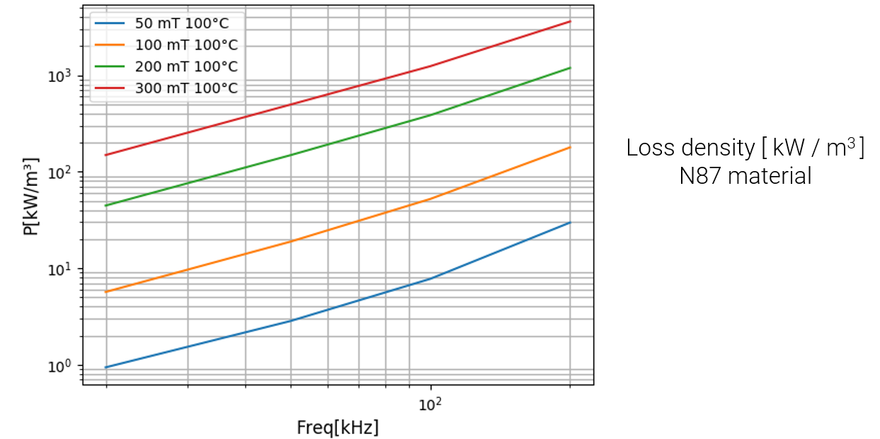
The core losses are computed from the core volume and the selected material’s loss density. This loss density depends on maximal induction \(B_{ACmax}\) and frequency f as shown in figure below:

4.1.2.1.5. Winding loss
The winding losses depend on the winding DC resistance value and the corrected value of the RMS current:
The DC resistance is based on the average turn length \(L_{turn}\) and the conductor section \(S_{conductor}\):
The value of the RMS current is corrected in order to take into account the difference between \(R_{AC}\) and \(R_{DC}\) (only a rough skin effect model is used, no proximity effect is modeled at all):
4.1.2.1.6. Cost
The cost of the inductors is calculated using the following formulation:
4.1.2.2. Design algorithm in auto design mode
The two steps of this approach are:
compute the minimum required area product from waveforms and other inputs such as loss densities,
compute a mass-optimal dimension set from this area product (as decribed in 1).
4.1.2.2.1. Area product relation
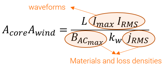
This relation, which allows estimating the minimum required area product \(A_c \times A_w\) is derived from:
a core relation: \(\Phi_{max} = L \times I_{max} = N_{turns} \times B_{ACmax} \times A_{core}\)
a winding relation: \(N_{turns} \times I_{rms} = k_w \times A_{wind} \times j_{RMS}\)

The area product formulation actually used by the design algorithm is slightly improved, taking into account:
increased AC winding losses via the corrected \(I_{RMS}\) described previously,
the derating of \(B_{ACmax}\) to values below \(B_{sat}\) because of core loss of the selected magnetic material.
If the selected magnetic material is (Most relevant), the magnetic material is auto-selected. For each magnetic
material, the maximum induction for the maximum loss density and given frequency at 100°C is estimated.
The material with the highest induction is then selected. If no public reference in the database suits
the design operating conditions, solutions include increasing the maximum core loss density,
sweeping through all magnetic materials to find a relevant reference, or adding a new private material.
Note that thermal design limitations are taken into account purely through target power densities:
winding loss density is linked to current density by the relation \(j_{RMS} = \sqrt{\frac{ Winding\ loss\ density}{\rho}}\) (with \(\rho\) the winding material’s resistivity) so the default value of 50 kW/m³ corresponds to roughly 1.5 A/mm²,
core loss density also has a default value of 50 kW/m³ which should be reasonable for medium-sized inductors without specific cooling-optimized construction.
4.1.2.2.2. Corrected \(I_{RMS}\)
For computing the corrected \(I_{RMS}\), the ratio \(R_ {AC} / R_ {DC}\) is assumed to be known a priori although it depends on the exact winding geometry which has not yet been determined at this point. In theory it is hardly justifiable, however:
a truly realistic estimate would require a fine consideration of the geometry, including in particular the 3D aspects,
this ratio does not play a major role in the dimensioning of (relatively low ripple) filtering inductances.
4.1.2.2.3. Derating of \(B_{ACmax}\)
For high ripples and/or switching frequencies, \(B_{ACmax}\) must be reduced to values significantly below \(B_{sat}\) in order to limit core loss density, as illustrated the figure below for different materials (extracted from 1).
.png)
4.1.2.2.4. Optimal mass dimensions
This second step aims to compute a set of 4 dimensions:
which optimizes the mass:
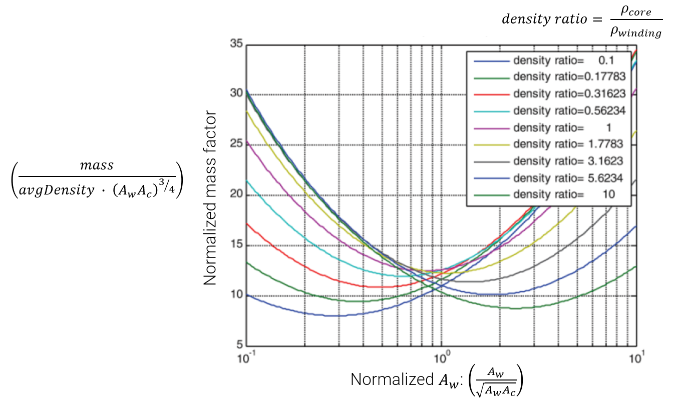
The figure below (extracted from 1) shows the normalized mass factor vs the normalized winding area: a family of curves corresponding to different density ratios are plotted to show that a minimum weight is obtained for different values of \(A_{wind}\). The interpretation is easily understandable: when the magnetic density is higher than conductor density (i.e. density ratio > 1, the right part of the figure), the proportion of magnetic material should be smaller thant the proportion of conductor material.

Actually, a numerical expression of \((A_{wind})_{opt}\) can be found:
As a result, the optimal dimensions are as follows:
4.1.3. The ideal and non-ideal transformer model
4.1.3.1. Models and assumptions
The ideal transformer model is the simplest available transformer model. The transformer is modeled as an electrical circuit with the following elements:
primary resistance (Rp)
secondary resistance (Rs)
ideal transformer with a transformer ratio (mTr)
If the non-ideal variant is selected, an additional magnetizing inductance is added in parallel of the ideal transformer the value of this inductance
Electrical schematic of the ideal transformer below
Electrical schematic of the non-ideal transformer below
The cost of a transformer is computed as:
4.1.3.2. Design algorithm in auto design mode
The auto-design approach for the transformer model is as follows:
the target transformer ratio is chosen by the user at the isolated tank level
2. the primary and secondary resistances are chosen so the resulting resistive power loss will be divided equally between primary and secondary with the following formulas:
volume is then computed as
with
\(\Phi_{max} = max(1.1 \cdot \int_{0}^{t} V_p(t) \,dt )\)
\(I_{rms\:rated} = I_{rmsPrimary} * 1.1\) the primary current rms value time a margin factor equal to 1.1
\(K_{volume}\) a factor related to the transformer technology
\(\alpha\) a correction factor. A dimensional analysis explains the default value of 3/4.
mass is derived as \(Mass = Volume \cdot Density\)
Note: In the case of the non ideal transformer model, the magnetizing inductance is provided by the user and does not affect the resulting Volume and Mass of the transformer