3.3. Cooling subsystem

Contents

• Cooling subsystem

  • No Cooling | Macrocell imposed temperatures

    • Junction temperature imposed

    • Case temperature imposed

    • Sink temperature imposed

  • Common thermal resistance

    • Parameters common to all variants

    • The R_th model

      • Manual configuration

      • Auto-design configuration

    • The Forced air fin heatsink model

      • Heatsink dimension

      • Thermal characteristics

      • Model and assumptions

        • Baseplate

        • Fins

      • Design algorithm in auto design mode

    • The Cold plate from library model

      • Cold Plate library

      • Thermal model

      • Additional characteristics

      • Design algorithm in auto design mode

The cooling subsystem is dedicated to the macrocell thermal management. There are two ways to use this subsystem:

• No cooling: the macrocell temperatures are imposed (\(T_{junction}\), \(T_{case}\) or \(T_{sink}\)):

  • Junction temperature imposed

  • Case temperature imposed

  • Sink temperature imposed

• Cooling model: the purpose is to cool the power switches of the conversion stage in order to keep them in their allowable temperature range despite power losses:

  • The Rth model

  • The Forced air fin heatsink model

  • The Cold plate from library model

3.3.1. No Cooling | Macrocell imposed temperatures

3.3.1.1. Junction temperature imposed

The following equivalent electrical schematic is used for this thermal model:

This model is the only model which doesn’t need an electrical and thermal coupled estimation.

Indeed, all the macrocell components (transistors and diodes) share the same junction temperature \(T_{junction}\). This temperature is used to estimate both conduction and switching losses, without considering the cooling.

Care must be taken with this model because the final design won’t consider any cooling.

3.3.1.2. Case temperature imposed

The following equivalent electrical schematic is used for this thermal model:

With this model, all the macrocell components (transistors and diodes) share the same case temperature \(T_{case}\).

Iterative process will then be used to find the junction temperature (and losses) of each component, to comply with the case temperature constraint.

The junction to case thermal resistance \(R_{th(j-c)}\) specified in the power switches libraries will be used for this model.

Care must be taken with this model because the final design won’t consider any cooling.

3.3.1.3. Sink temperature imposed

The following equivalent electrical schematic is used for this thermal model:

With this model, all the macrocell components (transistors and diodes) share the same sink temperature \(T_{sink}\).

Iterative process will then be used to find the junction temperature (and losses) of each component, to comply with the sink temperature constraint.

The case to sink thermal resistance \(R_{th(c-s)}\) specified in the macrocell subsystem will be used for this model.

Care must be taken with this model because the final design won’t consider any cooling.

3.3.2. Common thermal resistance

The following equivalent electrical schematic is used for this thermal model:

3.3.2.1. Parameters common to all variants

\(T_{cold \: source}\) is always imposed by the user.

All the feasible designs will reach the following requirements:

• The first condition verified is that the highest junction temperature \(T_{junction \: (highest)}\) of the macrocell subsystem doesn’t reach the maximum operating junction temperature \(T_{jOp(max)}\) (see power switch section):

  \(T_{junction \: (highest)} < T_{jOp \: (max)}\)

  • In manual configuration, \(T_{junction \: (highest)}\) is primarily considered an output of the system. It is calculated at the end of the design process and is used to verify whether the condition is met.

  • In auto-design configuration, \(T_{junction \: (highest)}\) is used as a cooling design constraint with the target margin temperature variable:

    \(T_{junction \: (highest)} = T_{jOp \: (max)} -\) Target margin temperature

• The other condition verified is that the Cooling system dissipation area is large enough to contain all the switch package areas, which is called the Cooled surface area:

  Cooling system dissipation area >= Cooled surface area

  

  • In manual configuration, the Cooling system dissipation area is imposed by the user, either directly in the

  sweep specification, or by selecting a component from the cold plate library.

  • In auto-design configuration, the Cooled surface area is a constraint:

    Cooled surface area \(=\) Total switch package areas \(\times ( 1 +\) Area margin \((\%))\)

    The Area margin accounts for the spacing between each component. Thus, the resulting Cooling system dissipation area will be least equal to this minimum surface.

3.3.2.2. The R_th model

This model is the simplest available for the cooling subsystem. The volume and the mass are directly linked to the value of \(R_{th(s-cs)}\).

3.3.2.2.1. Manual configuration

The user directly sets the values for volume and mass, as well as the \(R_{th(s-cs)}\) value. This variant is useful when a user already has a known cooling system and wants to check if the design is still feasible for another operating point for example.

3.3.2.2.2. Auto-design configuration

The \(R_{th(s-cs)}\) value is obtained by the design algorithm to satisfy the temperature condition mentioned above.

The volume and the mass of the cooling system are computed from user-provided coefficients, respectively \(Volume \times R_{th(s-cs)}\) and \(Mass \times R_{th(s-cs)}\). The following example gives the typical values for a given coldplate.

Technology	\(Volume \times R_{th(s-cs)} \: [m^{3}.°C/W]\)	\(Mass \times R_{th(s-cs)} \: [kg.°C/W]\)
Cold Plate	\(7.62\times10^{-6}\)	\(0.0135\)

How to determine those coefficients?

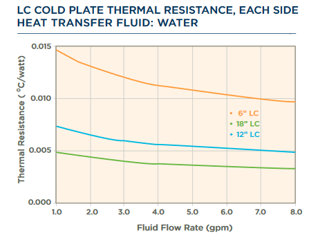
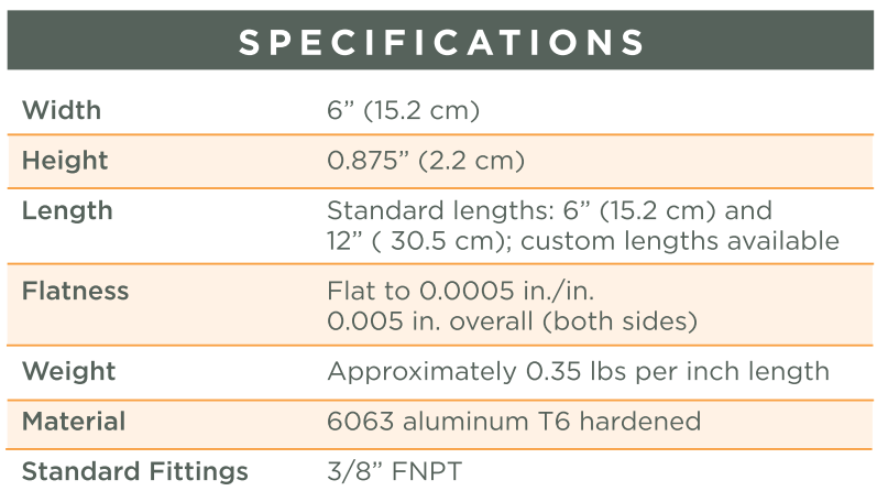
For example, for the default values of the cold plate, the coefficients are extracted from the data in the figures below:

The 6” long cold plate is used as reference at 1gpm flow rate. Based on the data:

\[Mass = 0.35 \times 6 = 2.1 \: lbs = 0.9 \: kg\]

\[Volume = 0.152 \times 0.152 \times 0.022 = 5 \times 10^{-4} \: m^{3}\]

\[R_{th} = 0.015 \: °C/W\]

\[Mass \times R_{th} \simeq 0.9 \times 0.015 = 0.0135 \: kg.°C/W\]

\[Volume \times R_{th} \simeq 5 \times 10^{-4} \times 0.015 = 7.62 \times 10^{-6} \: m^{3}.°C/W\]

3.3.2.3. The Forced air fin heatsink model

This model represents a forced air convection heatsink, constructed as a parallelepiped baseplate with straight parallel fins placed in an air flow with an imposed speed. Geometric parameters, along with parameters related to cooling conditions (such as fluid velocity), will be used to determine the \(R_{th(s-cs)}\) value.

3.3.2.3.1. Heatsink dimension

The next figure illustrates the main geometrical parameters used for the \(R_{th(s-cs)}\) estimation:

• z_baseplate: Baseplate thickness. A minimum value is usually necessary to ensure proper thermal spreading and for mechanical reasons.

• x_fin: Fin thickness following x direction. In auto-design mode, this value is automatically determined by the design algorithm.

• z_fin: Fin height following z direction. In auto-design mode, this value is automatically determined by the design algorithm.

• x_spacing: Air space between two fins. In auto-design mode, this value is automatically determined by the design algorithm.

• Fin number: Fin number. In auto-design mode, this value is automatically determined by the design algorithm.

• y: Heatsink dimension in the direction (along air flow). In auto-design mode, this value is automatically determined by the design algorithm.

• x: Heatsink dimension in the x direction (across fins).

• z: Heatsink dimension in the direction (along fins).

3.3.2.3.2. Thermal characteristics

• R_th(s-a): Heatsink-to-ambient thermal resistance.

• Cooled surface: Area of the thermal contact surface, i.e. mounting surface for the power switches being cooled.

3.3.2.3.3. Model and assumptions

The following figure illustrates the different thermal resistances from which we will calculate the R_th(s-a) thermal resistance.

with:

• \(R_{th\,conv}\) : thermal resistance which describes the heat exchange between the wall of the fin and the air stream (see Fins),

• \(R_{th\,baseconv}\) : thermal resistance which models the heat exchange by convection between the inter-fin spaces and the air (see Fins),

• \(R_{th\,accesfin}\) : thermal resistance of a fraction of the baseplate allowing to drain the heat towards a fin (see Baseplate),

• \(R_{th\,accesspace}\) : thermal resistance of a fraction of the baseplate allowing to drain the heat towards the inter-fin space (see Baseplate),

• \(R_{th\,fincond}\) : thermal resistance representing the conduction of heat in the fin (simple conduction model).

3.3.2.3.3.1. Baseplate

A homogeneous 1D heat flux is assumed in the baseplate. The lateral spreading resistance is neglected, which is acceptable if the surface of the heat source is close to that of the baseplate itself.

3.3.2.3.3.2. Fins

A fairly standard fin model such as described in this article is used.

The convective coefficient h is calculated from the geometry of the heatsink (inter-fin space in particular), from the properties of the materials and from the fluid (Prandtl, Reynolds and Nusselt numbers). The equivalent thermal resistance between the surface of the fins and the air stream can then be derived. The conduction resistance along the fin is taken into account.

The fluid is by default air at T_amb = 25°C and at atmospheric pressure (zero altitude).

3.3.2.3.4. Design algorithm in auto design mode

A heatsink matching the specifications and minimizing the mass is designed in this mode. In the context of this simple design, the baseplate is considered to have an squared shape to avoid dealing with the question of the arrangement of the components on the baseplate. The design algorithm is as follows:

1. The value of the thermal resistance (\(R_{th(spec)}\)) not to be exceeded is derived from :

   • the losses calculated in the components mounted on the heatsink,

   • the devices’ internal thermal resistances,

   • the maximum permissible temperatures of devices,

   • the ambient temperature.

2. The edge of the initial cooling surface is calculated as the square root of the total semiconductor package area (which does not guarantee a practical way of mounting these package to the heatsink baseplate),

3. Different combinations of number of fins, fin thickness and fin height are swept and the solution that optimizes the product \(R_{th} \cdot mass\) is chosen. The maximal fin height for the sweep will be determined either from the user defined limit or to not have a fin height larger than the baseplate width.

4. If \(R_{th(opt)}<R_{th(spec)}\), then a different proportion is looked (probably with fewer fins) which minimizes the mass and respects \(R_{th}<R_{th spec}\),

5. If \(R_{th(opt)}>R_{th(spec)}\) , the surface edge is increased and the parameters number of fins, fin thickness and fin height are swept to find solution with minimal mass. The surface is increased as long as the required \(R_{th(spec)}\) is not satisfied,

6. The various characteristics of the heatsink are displayed, in particular its total thermal resistance, its mass and its bounding volume.

3.3.2.4. The Cold plate from library model

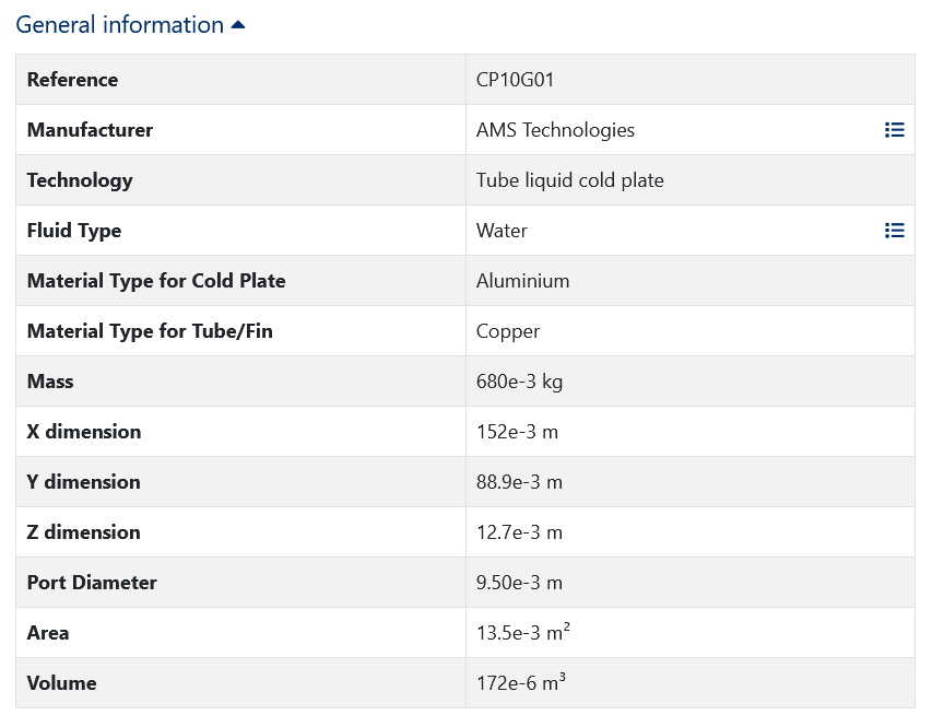
This model allows users to specify an off-the-shelf (data based) liquid cold plate. While PowerForge provides a few predefined references, users can also add their own private cold plate references. The model allows the user to specify the mass, dimensions, material type, fluid type, cost and to add coolant flow rate, thermal resistance and pressure drop data in the form of CSV files.

3.3.2.4.1. Cold Plate library

In the cold plate library, the existing references can be seen and accessed.

To add a new cold plate reference, click on “Create a private reference” and fill-in all the required parameters as presented in the figure below:

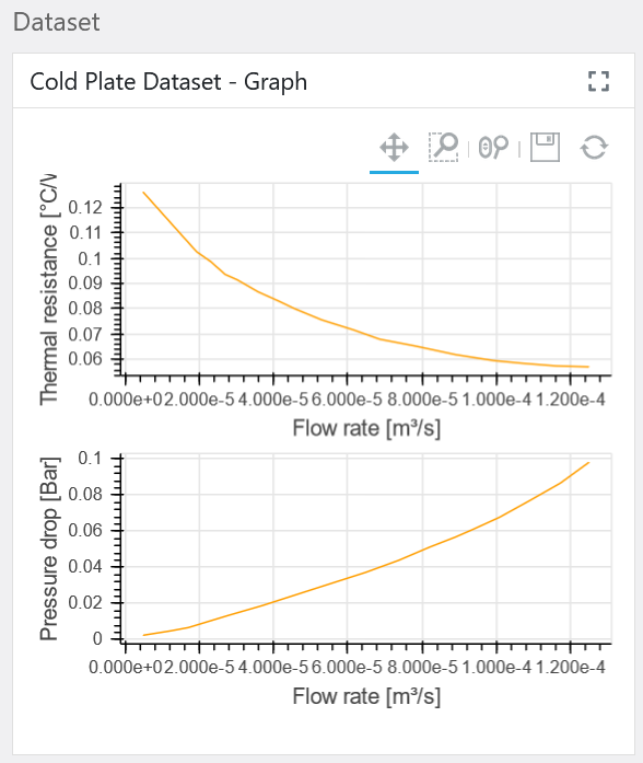
The data table need to be uploaded as a .csv file. The input data should have four columns: The first two columns should contain the coolant flow rate versus the thermal resistance data, the next two columns should contain the data for coolant flow rate versus pressure drop data.

The CSV file should use either comma (US/UK standard) or semicolon (EU standard) as the delimiter. An example file is available to download directly on the private reference form interface.

3.3.2.4.2. Thermal model

The cold plate model is a data-based model (not a physical model). The thermal model consists of a simple thermal resistance between the mounting surface for switches (thermal interface) and a cold source at the liquid temperature. The resistance value is a function of the flow rate. Flow rate outside the data bounds (min and max) is impossible and will result to a design failure (no extrapolation).

3.3.2.4.3. Additional characteristics

The pressure drop is also a function of the flow rate, so for each flow rate, a thermal resistance value and a pressure drop are given. The user can define a maximum allowed pressure drop and the design will fail if this pressure drop value is attained or exceeded.

The cold plate is supposed to be a one-side cold plate, and the modules are supposed to be placed in only one side of the cold plate. The design will be rejected if the total area of the power modules defined in the macrocell exceeds the cold plate cooling area. The modules are not actually placed on the cold plate, only a surface check is performed. Be aware that depending on the shape of the modules, the design can succeed but the modules may not necessarily all fit on the cold plate.

3.3.2.4.4. Design algorithm in auto design mode

1. Compute the minimum value of the thermal resistance (\(R_{th(target)}\)) needed to satisfy the input parameters based on

   • the losses calculated in the components mounted on the cold plate,

   • the devices’ internal thermal resistances,

   • the thermal interface’s thermal resistance,

   • the maximum permissible temperatures of devices,

   • the fluid temperature.

2. Use the data from the selected cold plate references to compute flow rate required to achieve the target thermal resistance. If \(R_{th(target)}\) value is above the maximal cold plate thermal resistance, usually at the minimal flow rate, then the minimal flow rate value is used, which can result in a much lower margin temperature than the target one. However, if \(R_{th(target)}\) is lower than the minimal thermal resistance, usually at the higher flow-rate, then the design is rejected.

3. Check if the selected cold plate(s) satisfy the requirements by comparing against the computed flow rate and pressure drop against the maximum allowed values. If the requirements are not met, the design is rejected.