2.2. Three phase DC/AC
Contents
2.2.1. Converter definition
A three-phase DC/AC converter (or inverter) performs bidirectional power conversion between a DC bus and a three-phase AC network (such as a grid or an electrical machine).
It is a voltage source inverter (VSI) structure, with 3 identical legs each connected to one of the AC phases. There is no neutral connection.
A positive (DC→AC) power flow corresponds to inverter operation and a negative (DC←AC) power flow corresponds to rectifier operation.
The reference power is defined on the AC side, hence total converter efficiency is computed by PowerForge as such:
if \(P_{AC}>0\) (inverter) then \(η = \dfrac { |P_{AC}| }{ |P_{AC}| + P_{loss} }\)
if \(P_{AC}<0\) (rectifier) then \(η = \dfrac { |P_{AC}| - P_{loss} }{ |P_{AC}|}\)
A three-phase DC/AC conversion stage is composed of several subsystems as shown below:
The total harmonic distortion of the phase-phase voltage at the bus interface and the line current are calculated using the following formulas:
where the sub-index 1 is for the fundamental and the rest the nth harmonic.
For the total weighted harmonic distortion of the phase-phase voltage:
2.2.2. Sources modeling
2.2.2.1. Ideal DC & AC sources
When using this operating point definition, the conversion stage’s DC interface is modeled as connected to an ideal DC source and its AC interface is modeled as connected to a balanced ideal 3-phase AC source. The natures of these sources depend on the order of the corresponding filters.
At the DC interface:
odd order filters will be connected to a current source,
even order filters will be connected to a voltage source.
At the AC interface:
odd order filters will be connected to a voltage source,
even order filters will be connected to a current source.
Transferred power is specified by PAC, the active power flowing out of the AC-side converter interface.
The sine AC voltage is specified by its fundamental frequency f0 and phase-to-phase RMS value UAC,0.
Designs with fsw / f0 > 5200 will be automatically unfeasible.
QAC reactive power is defined by:
cos φ: where φ is the angle between the phase-to-neutral voltage and current waveforms (amounting, with sine current waveforms, to the power factor)
QAC sign
2.2.2.2. Machine RLE
When using this operating point definition, the conversion stage’s DC interface is modeled as connected to an ideal DC source and AC interface is connected to a balanced 3-phase RLE model.
Transferred power is specified by Pemf, the active power used by the machine.
Qemf reactive power is defined by:
cos ψ: where ψ is the angle between the phase-to-neutral emf voltage and current waveforms (amounting, with sine current waveforms, to the power factor)
Qemf sign
2.2.2.3. Grid RLE
When using this operating point definition, the conversion stage’s DC interface is modeled as connected to an ideal DC source and AC interface is connected to a balanced 3-phase RLE model.
Transferred active and reactive power injected at the AC bus interface are specified by PAC and QAC. Passive sign convention is used, therefore if PAC and QAC, active and reactive power are positive, both powers are being injected into the grid.
Reference frame for angles is the phase neutral voltage of the E source as shown in the vector diagram.
2.2.2.4. Electrical machine with control
This operating point definition is made to allow the user to directly specify the operating point as a speed, torque and DC bus voltage (\(U_{DC}\)). In the system point of view, it is much easier to specify the target mecanical operating point than the electrical quantities. However, to convert the mechanical quantities to electrical ones, needed to perform the electrical simulation and design, the electrical machine model as well as the control strategies need to specified.

Available Machine Models:
Spatial harmonic model (only PMSM)
Available Controller Models:
2.2.2.4.1. Machine Models
The machine models are based on the models of femagtools (part of GT ecosystem) to allow a seamless and modeling continuity with GT-FEMAG (2D FEA machine design tool).
2.2.2.4.1.1. Permanent Magnet Synchronous Machine (PMSM)
The PMSM models :”PMSM model (no dependencies)” and “Machine form library” share the same common modeling. The main difference between the models lies in how the model parameters are defined. Indeed, the “PMSM model (no dependencies)” model only use scalar value as model input whereas the “Machine form library” model uses Ld/Lq/psim maps from FEA analysis.
Electrical modeling
The machine electrical modeling is a current source. Indeed, for the inverter simulation, the machine is simulated as a pure sine current source at the fundamental frequency.
Torque equation
With
\(\psi_{D} = L_D \cdot I_D + \sqrt{2} \cdot \psi_M\) the flux over the D axis
\(\psi_{Q} = L_Q \cdot I_Q\) the flux over the Q axis
\(m\) the number of phases
\(p\) the number of pole pairs
\(L_D\) and \(L_Q\) the inductance value in the D and Q axis. These values are scalar in PMSM no dependencies model or a lookup tables in the PMSM from library model
\(\psi_M\) the flux linkage. This value is scalar in PMSM no dependencies model or a lookup tables in the PMSM from library model
The \(L_D\), \(L_Q\) and \(\psi_M\) lookup tables are function of (\(I_D\), \(I_Q\), \(T_{Rotor}\))
Voltage equations
With
\(R_{DCstator}(20°C)\) the stator DC resistance given at 20°C
\(w = p \cdot speed \cdot \frac{2 \cdot \pi}{60}\) the electrical pulsation in rad/s
Copper loss calculation
The copper losses of a PMSM is stator copper loss so \(P_{Cu}\) is defined as:
with the AC resistance \(R_{AC}\) defined as:
with
\(k_{th}=0.0039 °C^{-1}\) the temperature coefficient for Aluminum and Copper
\(k_{AC}(w)\) the AC coefficient factor function of the frequency defined as
with
and
Finally, the parameters used for the PMSM model are the following:
\(\gamma = 0.7\) constant coefficient
\(k_H = 2\) number of conductor in slot
\(\zeta = 0.2\) skin effect coefficient (penetration depth)
Iron and Magnet losses
Iron and Magnet losses are computed only if loss data are available in the machine data in the library (see machine from library section)
The total iron losses \(P_{Iron}\) is defined as
with
Magnet losses \(P_{IronMagnet}\):
Iron losses Stator \(P_{IronStator}\):
Iron losses of stator yoke \(P_{IronStatorYoke}\):
Iron losses of stator teeth \(P_{IronStatorTeeth}\):
Iron losses of rotor \(P_{IronRotor}\):
With:
\(f_{0ref}\) as the reference electrical frequency at which the loss lookup table have been computed (default: 50 Hz)
\(hs, hr, es, er\) as the power factor for hysteresis and eddy loss vs the frequency as detailed in table below
name |
detailed name |
default value |
|---|---|---|
hr |
Rotor hysteresis frequency loss factor |
1 |
hs |
Stator hysteresis frequency loss factor |
1 |
er |
Rotor eddy frequency loss factor |
2 |
es |
Stator eddy frequency loss factor |
2 |
\(f_{0}\) as the electrical frequency at which the losses are estimated
\(p\) the number of pole pairs
\(P_{HystStatorYoke}, P_{EddyStatorYoke}, P_{HystStatorTeeth}, P_{EddyStatorTeeth}, P_{HystRotor}, P_{EddyRotor}, P_{Magnet}\) are lookup tables stored in the Machine library and provided by the user.
The lookup tables are function of (\(I_D\), \(I_Q\), \(T_{Rotor}\)).
Temperature Interpolation
Each lookup tables used in the models above can be interpolated/extrapolated based on the temperature provided by the user. Both interpolation and extrapolation are linear.
Other Interpolation
The other lookup tables are NOT extrapolated and are interpolated with a spline function.
2.2.2.4.1.2. Electrically Exited Synchronous Machine (EESM)
The EESM model is available through the library devices. The model libray setup and requirements are explained in the library section. The main difference between the PMSM and the EESM model is that the EESM model uses \(\psi_{D}\) and \(\psi_{Q}\) maps instead of \(L_D\) and \(L_Q\) maps.
Electrical modeling
The machine electrical modeling is a current source. Indeed, for the inverter simulation, the machine is simulated as a pure sine current source at the f0 frequency.
Torque equation
With
\(\psi_{D}\) the flux over the D axis is a lookup tables in the EESM from library model function of (\(I_D\), \(I_Q\), \(I_{Ex}\))
\(\psi_{Q}\) the flux over the Q axis is a lookup tables in the EESM from library model function of (\(I_D\), \(I_Q\), \(I_{Ex}\))
\(m\) the number of phases
\(p\) the number of pole pairs
The voltage equations are defined above as (2), (3).
Copper loss calculation:
The copper losses of an EESM (\(P_{Cu}\)) are defined as:
with
\(P_{Cu,stator}\) the stator copper losses defined as (4)
\(P_{Cu,rotor}\) the rotor copper losses defined below (11). The Rotor current is supposed to be only DC
with \(R_{DC,Rotor}\) a function of the rotor temperature
Iron losses
The iron losses are computed only if loss data are available in the machine data in the library (see machine from library section)
The total iron losses \(P_{Iron}\) is defined as
with
Temperature Dependance
The lookup tables of this model are not dependent over the temperature. Only the \(R_{DC,Rotor}\) and \(R_{AC,Stator}\) are temperature dependant
Interpolation and extraploation
The lookup tables of the EESM model are NOT extrapolated. The interpolation is linear.
2.2.2.4.1.3. Spatial harmonic model (PMSM)
The spatial harmonic model allows one to capture the harmonic content of the line current generated by the inverter (modulation strategy, switching frequency) and by the machine itself (reluctant torque, …)
The first step to use this model is to use GT-FEMAG, a finite element electromagnetic modeling tool built for motor design to design a motor. After the motor design has been finalized, GT-FEMAG can export a very high-fidelity parameter map model of the motor. These flux maps in the d and q axis are a function of the Id, Iq and rotor position. These maps are transformed to lookup tables and inverted in order to make the PMSM model described in the figure below.

The following equations are solved at each time-step
With
\(\theta\) the electrical machine angular position
\(f^{-1}\) and \(g^{-1}\) the inverse lookup tables from the FEA analysis
The torque function (9) is also solved at each time-step.
The control of this model is simulated in open-loop. The control parameters are estimated the same way as the other machine models and are presented in the section below.
The simulation output different quantities:
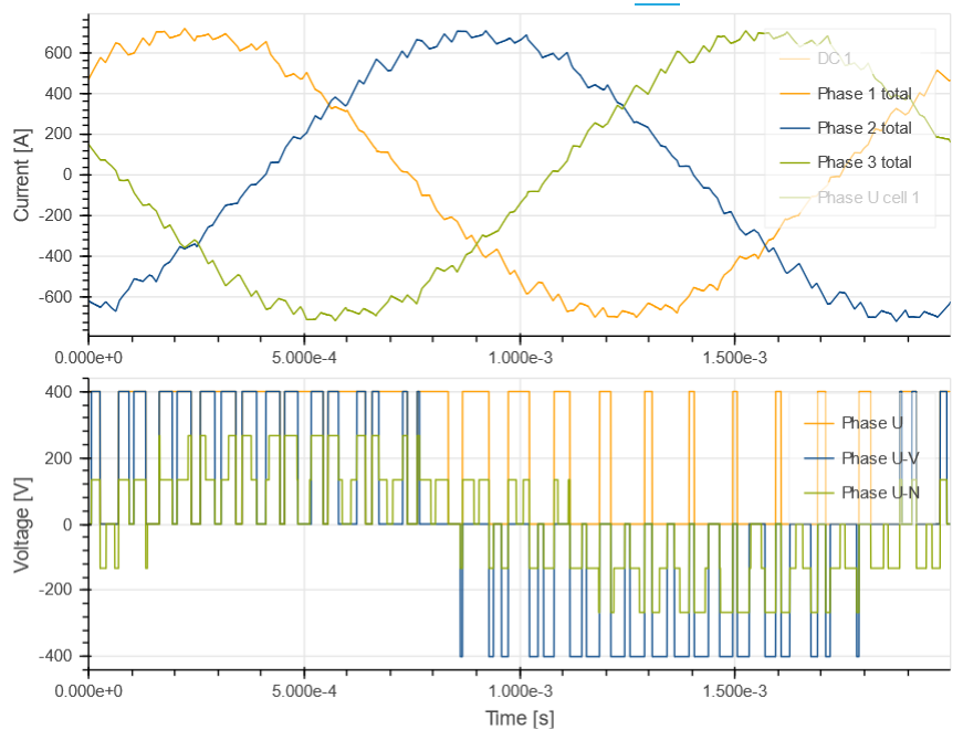
The machine phase currents waveforms -> available in the Macrocell tab
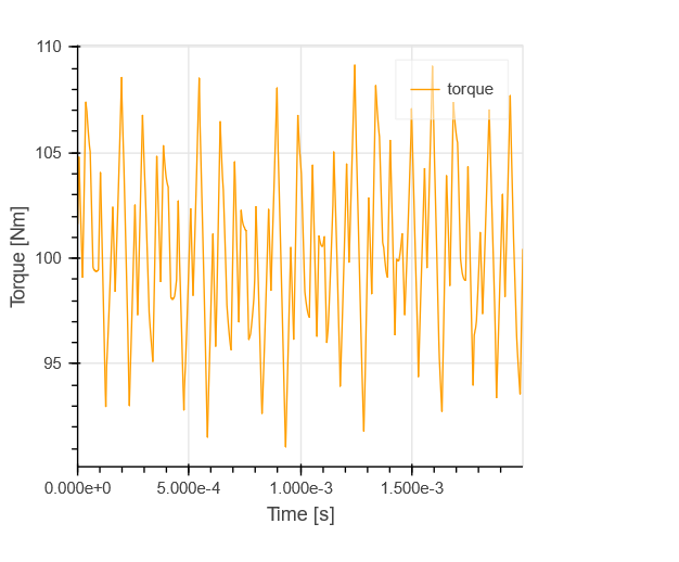
The torque waveforms -> available in the Operating point > Machine tab
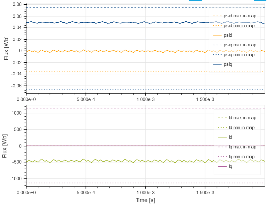
The flux waveforms (\(\psi_{D}, \psi_{Q}\)) -> available in the Operating point > Machine tab
Note
Depending on the stator resistance, the simulation can have a small low frequency oscillation that is only a simulation artifact. As a result, the torque ripple and torque ripple ratio can be a little bit overestimated. In addition the average torque can also deviate from the target torque value.
The waveforms can be downloaded as a CSV file in any figure.
Phase currents |
Torque |
Flux (D, Q) |
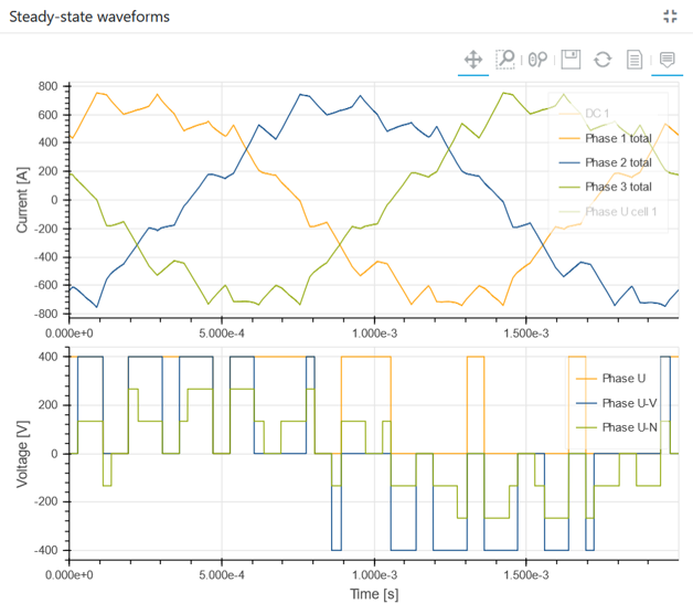
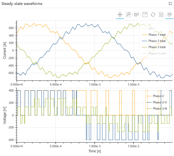
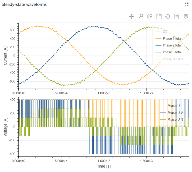
The switching frequency impact on the motor current ripple (and thus torque) can be analysed. An example is shown below with three different switching frequencies.
\(f_{sw} = 3kHz\) |
\(f_{sw} = 6kHz\) |
\(f_{sw} = 20kHz\) |
The currents can be used in GT-FEMAG to estimate the machine losses as well as the mechanical forces for an NVH workflow. Please contact an application engineer if you want to know more about this workflow with GT-FEMAG.
2.2.2.4.2. Controller Models
The controller are the way the electrical machines are piloted. The controllers solve a minimization under constraint function to find the electrical quantities used to control the machine at the target operating point.
The controller find the electrical control parameters to operate the electrical machine at the target speed and torque while doing it as efficiently as possible.
Two controllers variant are available:
Minimize stator current (MTPA + FW)
Minimize copper losses
The input for the controllers are the following:
- \(I_{Rated,RMS} (A)\): the maximum RMS current in a phase.
It is often defined by analysing the machine thermal limits. In PowerForge, this value must not exceed the maximum current value in the maps for the “Machine from library” and “Spatial harmonic model” variants.
- Maximum speed (RPM): the maximum speed of the machine.
The target speed must not exceed this value otherwise the model will fail. It is also used to make the maximum torque curve in the design dashboard as the curve limit.
- \(k_{voltage}\): the output voltage ratio.
The quantities is used to calculate the maximum available output voltage defined as \(V_{MAX} = k_{voltage} \cdot G_{MAX} \cdot V_{DC}\) with \(G_{MAX}\) maximum inverter gain. This maximum gain depends on the modulation strategy used (sine modulation: 1, homopolar injection: \(2 / \sqrt{3}\), over-modulation: \(4 / \pi\)
2.2.2.4.2.1. Minimize stator current (MTPA + FW)
As said in the name, this controller aim at minimizing the line current. This method is often called Maximal Torque Per Ampere (MTPA). This same minimization problem will automatically shift toward Field Weakening (FW) and Maximal Torque Per Volt (MTPV) when the target maximal current is reached.
With
2.2.2.4.2.2. Minimize copper losses
As said in the name, this controller aim at minimizing the copper losses. This minimization problem will automatically shift toward Field Weakening (FW) and Maximal Torque Per Volt (MTPV) when the target maximal torque is reached.
This is the preferred controller if an EESM is used. This controller variant is giving the same results as the Minimize stator current for a PMSM model.
With
\(P_{Cu}\) defined as (4) for a PMSM and as (10) for an EESM
\(X = [I_Q, I_D]\) for a PMSM and \(X = [I_Q, I_D, I_{Ex}]\) for an EESM
\(T(X)\) is the torque function (9)
\(V_{AC,RMS}(X) = \sqrt{\frac{V_Q^2(X) + V_D^2(X)}{2}}\) with \(V_Q\) and \(V_D\) defined in (2) (3)
\(I_{AC,RMS} = \sqrt{\frac{I_Q^2 + I_D^2}{2}}\)
